Configuring Round Robin Databases and Archives
We mentioned in the previous section that the Cacti application stores management data in a Round Robin Database (RRD) using the tools and utilities provided by the rrdtool application. In this section we shall examine in more detail the concepts required to create Round Robin Databases (RRDs) suitable for storing the data you desire for the required time period with the minimum of overhead.
More detailed information may be found in the official RRDtool documentation◳.
Consolidation functions
| Time | Temperature |
|---|---|
| 0 | 28 |
| 60 | 29 |
| 120 | 27 |
| 180 | 31 |
| 240 | 34 |
| 300 | 29 |
| 360 | 27 |
| 420 | 28 |
| 480 | 30 |
| 540 | 29 |
When data is inserted into almost any modern database it is usually stored in some kind of structure, often referred to as a table. Usually tables may contain more than one field for each record. In the example (right) we have a table consisting of two fields. The first is a time value (starting at zero for convenience) and the second is a temperature reading (presumably retrieved from a sensor of some kind).
There are two obvious limitations however to storing data in this manner. The first is that as more data is added the table takes up more storage space. The second is that to store such data over a long period of time requires a vast number of records (527,040 rows for one minute samples for one year). The Round Robin Database (RRD) is designed to overcome both of these limitations.
The first limitation is overcome by simply discarding the oldest data from the table as new data is added. In this way a Round Robin Database (RRD) maintains a constant size allowing us to ensure the storage requirements of the system are met in advance.
The second limitation is overcome by taking advantage of the fact that we don't usually require high resolution archive data. When examining the temperature of a device over a long period, one year for example, it is still desirable that the temperature was measured as often as possible to ensure that we captured all the moments of interest. What we probably don't need however is to see every single one of those measurements.
| Time | Temperature | ||
|---|---|---|---|
| Min | Max | Avg | |
| 240 | 27 | 34 | 29 |
| 540 | 27 | 30 | 28 |
We can therefore compress, or consolidate, the original data into a more compact form by extracting the interesting information such as the minimum, maximum and average values of several samples and then storing these in another table. The example table (left) shows the above data consolidated into just two rows, one for every five minutes of the original data. This additional table is often referred to as a Round Robin Archive (RRA).
Clearly, for this type of consolidation to be possible the previous level table must contain at least the number of rows which will be consolidated. If the previous level table contains more rows than are required to perform the consolidation they may still be used when higher resolution data is required from the database. If the same time period is covered by data from more than one level rrdtool will automatically use the highest resolution data.
The rrdtool application defines four consolidation functions which may be used to compress stored data named maximum, minimum, average and last. The function of each should be fairly obvious after the above description so we shall not elaborate further here however more information is available in the rrdtool documentation.
Instantaneous or Time-Integral data
Before we continue it is worth briefly mentioning the two distinct types of data which can be collected and graphed by the Cacti application.
- The first type of data is often referred to as an instantaneous value. A temperature sensor or the number of running processes are both good examples of this as they both provide a single value captured at the moment of sampling. It should be noted that any instantaneous value is precisely that, a single value sampled at that instant, it does not provide a minimum, maximum or average value since the last measurement was taken.
- The second type of data is commonly referred to as a time-integral value. A good example of such data is the number of packets transmitted over a network interface since the last sample. Unlike an instantaneous value a time-integral value provides an average value calculated by dividing the difference between the number returned and the previous sample by the time since the last sample, it does not provide a minimum, maximum or instantaneous value.
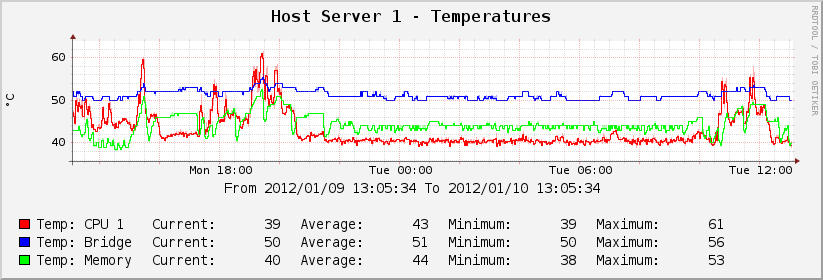
It is sometimes convenient when creating graphs using Cacti to ignore the above statements however and use an instantaneous value as an average value enabling graphs such as those below to be generated from the same Round Robin Database (RRD) with the minimum of storage and processing overhead. It is important to remember that doing so does not make it so and although the graphs will be produced correctly the first graph is in fact showing instantaneous values and not the average values.
As you can see in the graph below, Figure 2.1 [A graph of three temperature measurements over one day], the instantaneous values returned by three temperature sensors have been graphed simultaneously. We have chosen to store them as average values in the Round Robin Database (RRD) however so that we can make use of the same data on the next graph. As mentioned above it is important to always remember that the values being graphed are still instantaneous values however and so do not represent the true average value merely the value at that instant in time.
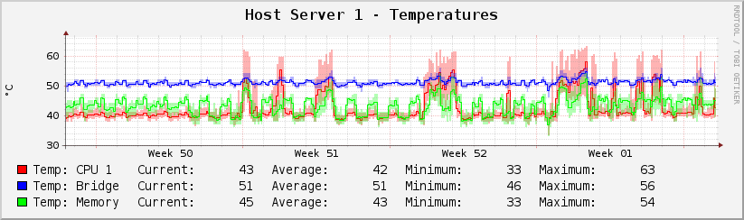
Whilst it is useful to graph the temperature of a device in the above manner when dealing with the measurements from a short period, just single day in our example, when dealing with larger ranges of time it is often useful to record the upper and lower bounds as well. In the graph below, Figure 2.2 [A graph of three temperature measurements over one month], we plot the average as a solid line and the range between the minimum and maximum values in a lighter shade. This allows both the average temperature of the device and the ranges of temperatures it has encountered to be observed at a glance.
Useful time calculations
To make the task of defining our Round Robin Databases (RRDs) as simple as possible we have prepared a short list of useful time calculations. The values presented here will be used in the next section when we actually create the Round Robin Databases (RRDs).
- Minutes in a day: 24 * 60 = 1440
- Minutes in a week: 1440 * 7 = 10080
- Minutes in a month: 1440 * 31 = 44670
- Minutes in a year: 1440 * 366 = 527040
- Minutes in ten years: 1440 * 366 * 10 = 527040 * 10 = 5270400
- Seconds in a day: 24 * 60 * 60 = 1440 * 60 = 86400
- Seconds in a week: 1440 * 7 * 60 = 10080 * 60 = 604800
- Seconds in a month: 1440 * 31 * 60 = 44670 * 60 = 2680200
- Seconds in a year: 1440 * 366 * 60 = 527040 * 60 = 31622400
- Seconds in ten years: 1440 * 366 * 60 * 10 = 527040 * 60 * 10 = 31622400 * 10 = 316224000
- Five minute intervals in a month: 44670 / 5 = 8934
- Hours in a year: 366 * 24 = 8784
- Days in ten years: 366 * 10 = 3660
If you would like to store your data for different time periods or with differing resolutions you may need to perform additional calculations.
Creating RRDs/RRAs
Assuming we wish to keep data with a resolution of one minute for one week we need to define an RRA with 10080 rows covering a time-span of 604800 seconds. As it is the first RRA it will have a step of one. Also, as it is the first level RRA it only makes sense to select either last or average as the consolidation function. Selecting more than one consolidation function for a first level RRA will not capture more data it will simply waste space by storing the same data multiple times.
Clearly, one week is hardly enough time to store data for analysis and trend-spotting purposes. We can define a second RRA to cover a period of one month storing data with a resolution of five minutes. As you can see from our calculation above this RRA will require 8934 rows and will cover a time-span of 2680200 seconds. As this RRA will store data with one fifth of the resolution of the first RRA a step of five should be chosen. As this is a second level RRA more than one consolidation function should probably be selected. A setting of maximum, minimum and average is most common.
In our experience, transient performance problems are often not noticed immediately. In several cases our clients have only noticed such issues after considerably more than a month has passed. To this end we store performance data with a resolution of one hour for a period of one year.
Using the information we have calculated above we can create a third RRA which will span the desired time-span of one year with a resolution of one hour. Such an RRA requires 8784 rows and covers a time-span of 31622400 seconds. As this RRA will only store one sample for every sixty collected by the first RRA we defined a step of sixty should be entered. As before three consolidation functions (maximum, minimum and average) are usually applied.
Finally, we would like to store data with a resolution of one day for a period of ten years. This is ideal for spotting long term trends which would otherwise be missed over a shorter period of time.
Again, using the values we have calculated above, we can define another RRA with the appropriate settings to cover a ten year period storing data at a resolution of one sample per day. Such an RRA would require 3660 rows, would cover a time-span of 316224000 seconds and would require a step value of 1440.